


Next: Approximation of the Test-Statistic
Up: Approximation of distribution function
Previous: Problem Formulation
In order to evaluate  for a given
  it is necessary to know the PDF (or the CDF) of the test-statistic
  .
While the PDF of the random variable is not known in analytical
closed form, the exact analytical expression of the statistical moments
of any order for the test-statistic monotonic function
.
While the PDF of the random variable is not known in analytical
closed form, the exact analytical expression of the statistical moments
of any order for the test-statistic monotonic function  can be found by using the well-known complex
Wishart distribution
for the matrix
can be found by using the well-known complex
Wishart distribution
for the matrix  given in [3]
|
|
|
|
(7) |
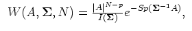
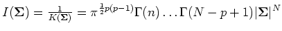
where
If the null hypothesis  is true, the matrix is
 distributed.
The  -th order moment of the random variable
can be straightforward determined from multidimensional
integral
|
![$\displaystyle \begin{array}{l}
M[V^h]=\int...\int\vert A\vert^h\frac{1}{\biggl(...
... _0,N)\times \ \times
\vert A\vert^{N-p}exp{[-Sp(\S _0^{-1}A)]dA}
\end{array}$](img44.png)
|
|
|
(8) |
The integration procedure is carry out here over area
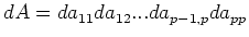 , where A are all
non-negative defined Hermitian
, where A are all
non-negative defined Hermitian ![$[p \times p]$](img46.png) matrices. The
integral (8) can be transformed into
matrices. The
integral (8) can be transformed into
|
![$\displaystyle \begin{array}{l}
M[V^h]=\frac {p^{hp}K(\S _0,N)} {K(\S _0,N+h)}\i...
...xp[-Sp(\S _0^{-1}A)]\}
\frac{1}{(\sum\limits_{i=1}^pa_{ii})^{ph}}dA
\end{array}$](img47.png)
|
|
|
(9) |
The element of integration (9) in figured
brackets is also Wishart distribution (7)
with  degrees of freedom
 . After
integration of (9) over all nondiagonal
distribution elements
. After
integration of (9) over all nondiagonal
distribution elements 
 , the partial joint distribution of the diagonal elements
 of the matrix is obtained. For
hypothesis this distribution is transformed into
product of one-dimensional distributions
of the matrix is obtained. For
hypothesis this distribution is transformed into
product of one-dimensional distributions
 . The one-dimensional complex Wishart
distribution
is the distribution
of the
. The one-dimensional complex Wishart
distribution
is the distribution
of the  -th diagonal element of the matrix . Note,
that
is
-th diagonal element of the matrix . Note,
that
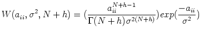
is  distribution
with
distribution
with  degrees of freedom:
|
|
|
|
(10) |
Thus, the expression for the -th order moment of the
test-statistic  can be reduced to the integral
![$M[V^h]=\underbrace{p^{hp}\frac{K(\S _0,N)}{K(\S _0,N+h)}}_{g}\int...\int
\frac{...
...}{{\bf\sigma}^2}}}{{\bf\sigma}^{2(N+h)}\Gamma(N+h)}
da_{11}da_{22}\dots da_{pp}$](img57.png)
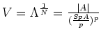
and can be represented as
![$M[V^h]=g<\frac{1} {(\sum\limits_{i=1}^pa_{ii}')^{ph}}> $](img58.png) ,
,
where  denotes expectation value.
Diagonal elements  of the matrix are
independent and identically distributed random
values with degrees of freedom and variances
of the matrix are
independent and identically distributed random
values with degrees of freedom and variances
 . Therefore, the random variable
 is
also distributed with
is
also distributed with  degrees of freedom.
Thereby, -th order moment of the random variable is
proportional to the
degrees of freedom.
Thereby, -th order moment of the random variable is
proportional to the  -th order moment
  of the
random variable
of the
random variable  which can be expressed through known
one-dimensional integral
which can be expressed through known
one-dimensional integral
|
![$\displaystyle \begin{array}{l}
M[B^r]=\int\limits_0^{\infty}B^r\frac{B^{(N+h)p-...
...c{{\bf\sigma}^{2Np}\Gamma(Np)}{{\bf\sigma}^{2(N+h)p}\Gamma((N+h)p)}
\end{array}$](img67.png)
|
|
|
(11) |
For practical calculations of the high order moments of the
test-statistic it is conveniently to transform the last
expression into product using properties of gamma-function:
![$M[V^h]=g\frac{{\bf\sigma}^{2pN}\Gamma(pN)}{{\bf\sigma}^{2p(N+h)}\Gamma(p(N+h))}...
...\times\ \times\frac
{\Gamma(N+h)...\Gamma(N+h-p+1)}{\Gamma(N)...\Gamma(N-p+1)}$](img68.png)
So, the exact analytical expression for the -th order moment of the test-statistic is
|
![$\displaystyle M[V^h]=
p^{hp}\frac{\prod\limits_{i=1}^{p}\prod\limits_{j=1}^{h}(j+N-i)}{\prod\limits_{i=1}^{ph}(i+pN-1)}$](img69.png)
|
|
|
(12) |
It is easy to see that the distribution of the random
variable is concentrated in interval [0,1]. So, there
are moments of any order (12) for , and
they completely determine its distribution
function [5]. It is worth to notice that the
characteristic function of the random variable is
expressed through moments as a converging Taylor series.
Next: Approximation of the Test-Statistic
Up: Approximation of distribution function
Previous: Problem Formulation